Measures of Center
Section 3.1Compute the mean and median of a data set
Mean of a Data Set
The mean of a data set represents its center. It’s like the balance point where all the data values, viewed as weights, would even out.
The beam levels at 81.2, and that is the mean of the five scores.
 Definition
Notation - Population Versus Sample
A population includes all individuals of interest, while a sample is a smaller group taken from the population. The mean is calculated the same way for both, but the notation is different.
DefinitionComputing the Mean
Given a list of numbers , the sample mean is computed as:
… and the population mean is computed as:
Median of a Data Set
The median is a measure of center that divides an ordered data set in half, with half the values below it and half above it. The method to calculate the median varies depending on whether the number of observations is even or odd.
If is odd, the median is the middle number.
If is even, the median is the average of the two middle numbers.

 Example
Example: Computing the Mean and Median
During a semester, a student took five exams. The population of exam scores is 78, 83, 92, 68, and 85. Find the mean and median of the exam scores.
Arrange the data values in increasing order.
68 78 83 85 92The median is the middle number, 83.
 Example
Example: Median with Even Number of Values
Eight patients undergo a new surgical procedure, and the number of days spent in recovery for each is as follows. Find the median number of days in recovery.
20 15 12 27 13 19 13 21Arrange the data values in increasing order.
12 13 13 15 19 20 21 27The median is the average of the two middle numbers.
 Calculator
1-Var Stats Command
The 1-Var Stats command in the TI-84 Plus calculator displays a list of the most common parameters and statistics for a given data set. This command is accessed by pressing STAT and then highlighting the CALC menu.
CalculatorExample: Mean and Median with 1-Var Stats
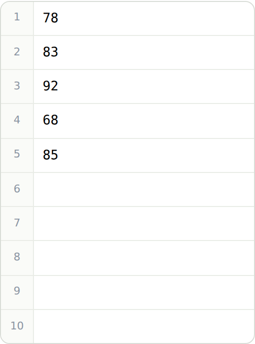
The same five exam scores, 78, 83, 92, 68, and 85, are entered in list L1. Then 1-Var Stats is selected from the STAT ▸ CALC menu.
The data in L1
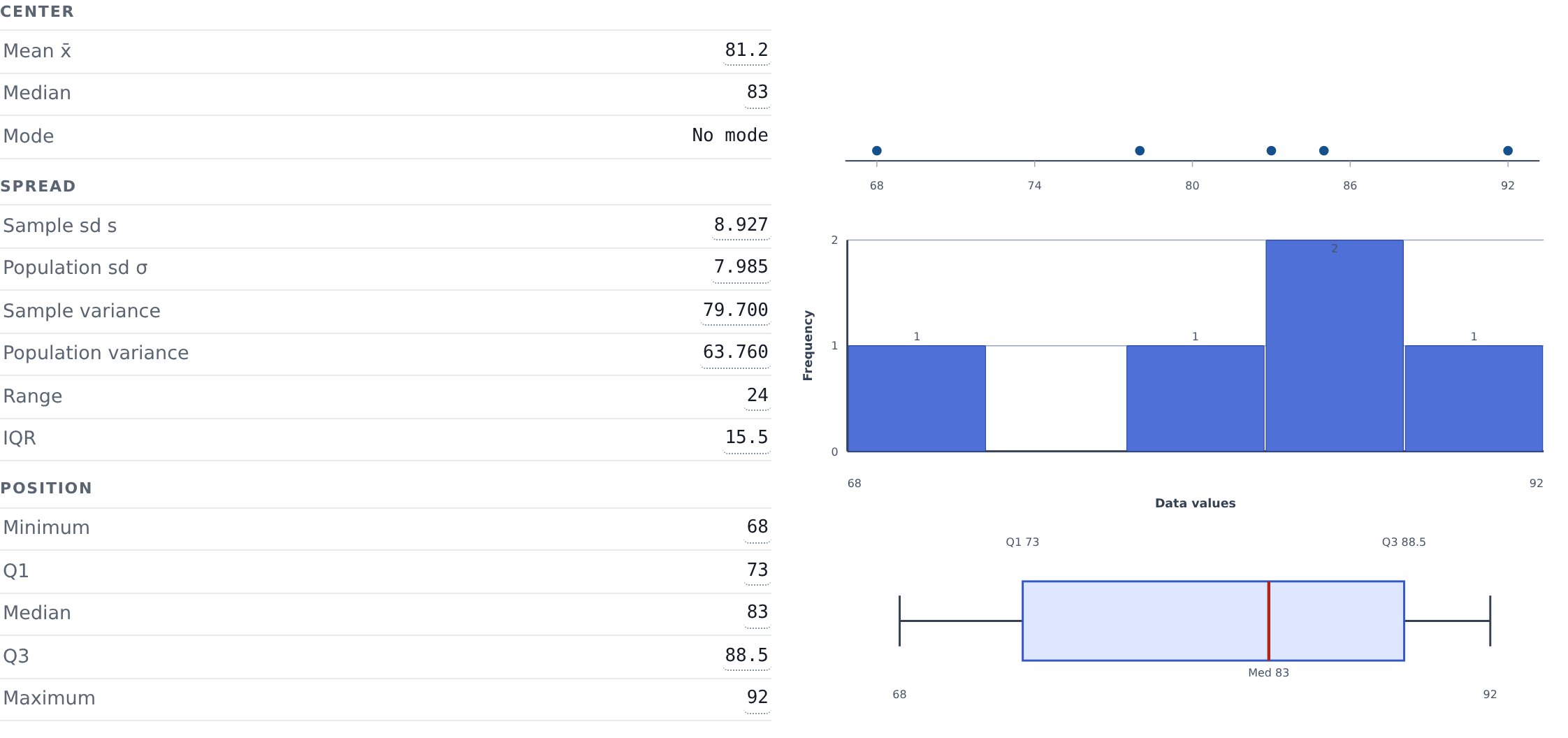
1-Var Stats output
Scrolled down for the median
The calculator gives the mean as 81.2 and the median as 83, the same values found by hand. These five scores are the entire population, so the mean it reports is the population mean.
 Interactive
The Complete Statistics Calculator
barrymonk.com/stats-calculator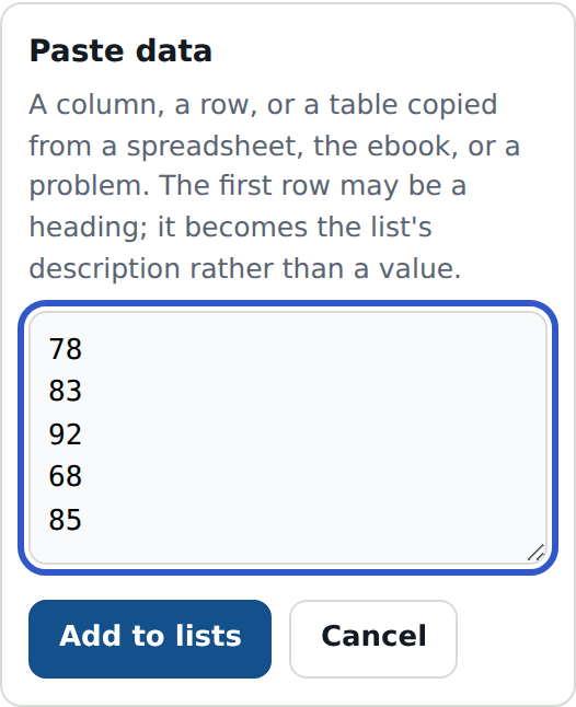
 Interactive
Running 1-Var Stats in the Calculator

Compare properties of the mean and median
The Mean is More Influenced by Extreme Values
Both the mean and median are measures of center. However, the mean is more influenced by extreme values than the median.
A statistic is considered resistant if it is not significantly affected by extreme values. The median is resistant, while the mean is not.
 Example
Example: The Median is Resistant
Five families had annual incomes of $25,000, $31,000, $34,000, $44,000, and $56,000. The family earning $25,000 won the lottery, and their income jumped to $1,025,000.
Before the lottery win, the mean and median are as follows.
After the lottery win, the mean and median are as follows.
The extreme income of $1,025,000 significantly raised the mean from $38,000 to $238,000, while the median only increased from $34,000 to $44,000, showing the median’s resistance to extreme values.
Mean, Median, and the Shape of a Data Set
The mean and median measure the center of a data set in different ways.
The mean and median are equal.
There are large values in the right tail. The mean is often greater than the median.
The mean is often less than the median.
 Check Your Understanding
Skewed to the right, skewed to the left, or approximately symmetric?
A café tracks customers served in its first hour each day. The mean is 11 and the median is 4.
Skewed to the rightA hobby club records weekly hours members spend on projects. The mean is 4 hours and the median is 12 hours.
Skewed to the leftA study finds car owners drive a mean of 801 miles per year with a median of 798 miles.
Approximately symmetricFind the mode of a data set
 Definition
Mode of a Data Set
A value that is sometimes classified as a measure of center is the mode.
The mode of a data set is the value that appears most frequently.
If two or more values are tied for the most frequent, they are all considered to be modes.
If the values all have the same frequency, we say that the data set has no mode.
 Example
Example: Mode of a Data Set
Ten students were asked how many siblings they had. The results, arranged in order, were 0, 1, 1, 1, 1, 2, 2, 3, 3, 6. Find the mode of this data set.
0 1 1 1 1 2 2 3 3 6The value that appears most frequently is 1. Therefore, the mode is 1.
Mode – Measure of Center?
The mode is sometimes classified as a measure of center. However, this isn’t really accurate. The mode can be the largest value in a data set, or the smallest, or anywhere in between.
Mode for Qualitative Data
Means and medians apply only to quantitative data, while the mode can be computed for both qualitative and quantitative data.
Following is a list of the makes of all the cars rented by an automobile rental company on a particular day. Which make of car is the mode?
The most frequent category is “Toyota,” which appears six times.
| Honda | Toyota | Toyota | Honda | Ford |
| Chevrolet | Nissan | Ford | Chevrolet | Chevrolet |
| Honda | Dodge | Ford | Ford | Toyota |
| Chevrolet | Toyota | Toyota | Toyota | Nissan |
Three measures of center
The mean of a data set represents its center. It’s like the balance point where all the data values, viewed as weights, would even out.
The median is a measure of center that divides an ordered data set in half, with half the values below it and half above it.
The median is resistant, while the mean is not.
The mode of a data set is the value that appears most frequently.
Measures of Spread
Section 3.2San Francisco vs. St. Louis
Suppose you were deciding between living in San Francisco and St. Louis. One thing you might consider is weather. The table presents the average monthly temperatures, in degrees Fahrenheit, for both cities.


| Jan | Feb | Mar | Apr | May | Jun | Jul | Aug | Sep | Oct | Nov | Dec | |
| San Francisco | 51 | 54 | 55 | 56 | 58 | 60 | 60 | 61 | 63 | 62 | 58 | 52 |
| St. Louis | 30 | 35 | 44 | 57 | 66 | 75 | 79 | 78 | 70 | 59 | 45 | 35 |
The mean temperatures are similar: 57.5° for San Francisco and 56.1° for St. Louis. However, St. Louis has more temperature variation.
The mean shows the center, but we also need to measure the spread to fully describe the data set.
Compute the range of a data set
Range of a Data Set
The range is a simple way to measure spread. The range of a data set is the difference between the largest value and the smallest value.
| Jan | Feb | Mar | Apr | May | Jun | Jul | Aug | Sep | Oct | Nov | Dec | |
| San Francisco | 51 | 54 | 55 | 56 | 58 | 60 | 60 | 61 | 63 | 62 | 58 | 52 |
| St. Louis | 30 | 35 | 44 | 57 | 66 | 75 | 79 | 78 | 70 | 59 | 45 | 35 |
The range of the San Francisco temperatures is: 63 − 51 = 12.
The range of the St. Louis temperatures is: 79 − 30 = 49.
Although the range is easy to compute, it is not often used in practice because it only involves two values from the data set.
Compute the variance of a population and a sample

The Variance
When a data set has little spread, most values are close to the mean. With more spread, values are farther from the mean. Variance measures how far, on average, data values are from the mean.
Variance is calculated differently for populations and samples.
DefinitionPopulation Variance
ExampleExample: Population Variance
Compute the population variance for the San Francisco temperatures.
| Jan | Feb | Mar | Apr | May | Jun | Jul | Aug | Sep | Oct | Nov | Dec | |
| 51 | 54 | 55 | 56 | 58 | 60 | 60 | 61 | 63 | 62 | 58 | 52 | |
| −6.5 | −3.5 | −2.5 | −1.5 | 0.5 | 2.5 | 2.5 | 3.5 | 5.5 | 4.5 | 0.5 | −5.5 |
ExampleExample: Population Variance
| Jan | Feb | Mar | Apr | May | Jun | Jul | Aug | Sep | Oct | Nov | Dec | |
| 51 | 54 | 55 | 56 | 58 | 60 | 60 | 61 | 63 | 62 | 58 | 52 | |
| −6.5 | −3.5 | −2.5 | −1.5 | 0.5 | 2.5 | 2.5 | 3.5 | 5.5 | 4.5 | 0.5 | −5.5 | |
| 42.25 | 12.25 | 6.25 | 2.25 | 0.25 | 6.25 | 6.25 | 12.25 | 30.25 | 20.25 | 0.25 | 30.25 |
DefinitionSample Variance
When computing sample variance, the sample mean is used for deviations. Deviations using the sample mean are typically smaller than those using the population mean.
If we divided by when calculating sample variance, it would generally be smaller than the population variance. To correct this, we divide the sum of squared deviations by instead.
ExampleExample: Sample Variance
A new type of battery is being tested for laptop computers. The lifetimes, in hours, of six batteries, are 3, 4, 6, 5, 4, 2. Find the sample variance of the lifetimes.
We find the sample mean to be 4. The sample variance is:
Two measures of spread
The range of a data set is the difference between the largest value and the smallest value.
Variance measures how far, on average, data values are from the mean.
To correct this, we divide the sum of squared deviations by instead.