Least Squares Regression and Correlation
Section 4.1 & 4.2
Construct scatterplots
Suppose that a real estate agent wants to study the relationship between the size of a house and its selling price. It is reasonable to suspect that the selling price is related to the size of the house. Specifically, we expect that houses with larger sizes are more likely to have higher selling prices.
A good way to visualize a relationship like this is with a scatterplot. In a scatterplot, each individual in the data set contributes an ordered pair of numbers, and each ordered pair is plotted on a set of axes.
The Data
| Size (Square Feet) | Selling Price ($1000s) |
|---|---|
| 2521 | 400 |
| 2555 | 426 |
| 2735 | 428 |
| 2846 | 435 |
| 3028 | 469 |
| 3049 | 475 |
| 3198 | 488 |
| 3198 | 455 |
 Calculator
Constructing a Scatterplot
The following steps will create a scatterplot for the house sizes and prices data using the Statistics Calculator at barrymonk.com/stats-calculator.
Step 1: Enter the eight sizes in L1 and the eight prices in L2.
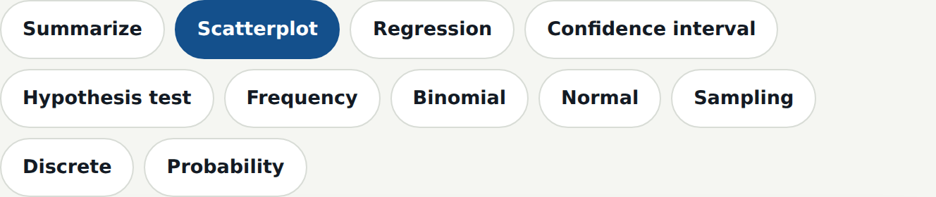
Step 2: Choose Scatterplot from the tool strip.
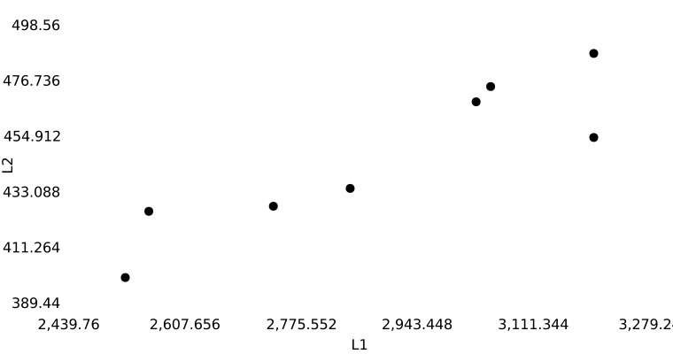
Step 3: Set x values to L1 and y values to L2, then press Run.
Positive Linear Association
Observe that larger sizes tend to be associated with larger prices, and smaller sizes tend to be associated with smaller prices. We refer to this as a positive association between size and selling price.
In addition, the points tend to cluster around a straight line. We describe this by saying that the relationship between the two variables is linear.
Therefore, we can say that the scatterplot exhibits a positive linear association between size and selling price.
 Definition
Other Types of Association
Two variables are positively associated if large values of one variable are associated with large values of the other.
Two variables are negatively associated if large values of one variable are associated with small values of the other.
Two variables have a linear relationship if the data tend to cluster around a straight line when plotted on a scatterplot.
 Check Your Understanding
State the type of association that is exhibited:
Choices: positive linear, negative linear, positive nonlinear, negative nonlinear, weak or no association.
 Definition
Correlation Coefficient
When two variables have a linear relationship, we want to measure how strong the relationship is. A numerical measure of the strength of the linear relationship between two variables is called the correlation coefficient.
Properties of the Correlation Coefficient
The correlation coefficient is always between −1 and 1. That is, .
The correlation coefficient does not depend on the units of the variables.
It does not matter which variable is x and which is y.
The correlation coefficient only measures the strength of the linear relationship. It can be misleading when the relationship is nonlinear.
Interpreting the Correlation Coefficient
the two variables have a positive linear association.
the two variables have a negative linear association.
the linear association is weak.
The closer is to 1, the more strongly positive the linear association is.
The closer is to −1, the more strongly negative the linear association is.
Correlation Coefficient with Technology
There is a strong positive linear relationship between size and selling price.
The Correlation Coefficient is Not Resistant
A statistic is resistant if its value is not affected much by extreme values (large or small) in the data set. The correlation coefficient is not resistant.
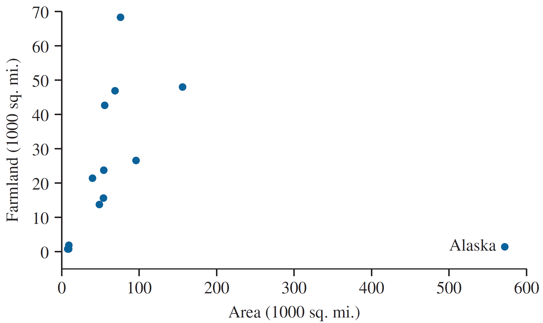
The plot shows area of farmland versus total land area for a selection of U.S. states. Alaska is an outlier. Because of the outlier, the correlation coefficient for this plot is −0.119, which is misleading. If the outlier is removed, the correlation coefficient for the remaining points is = 0.710.

 Interactive
Correlation Explorer
Drag any house. The correlation coefficient is recomputed as it moves.
 Think About It
Correlation is Not the Same as Causation!

Correlation: 99.79% ( = 0.99789126)

Correlation: 94.71% ( = 0.947091)

The Least-Squares Regression Line
DefinitionLeast-Squares Regression Line
We want to find the line that “best fits” the data.
This line is called the Least-Squares Regression Line.
CalculatorComputing the Least-Squares Regression Line
The following steps compute the least-squares regression line for the house size and selling price data using the Statistics Calculator at barrymonk.com/stats-calculator.
Step 1: Choose Regression from the tool strip.
Step 2: Set Explanatory variable x to L1 and Outcome variable y to L2.
Step 3: Press Run. The command bar composes LinReg(a+bx) L1,L2.
 Calculator
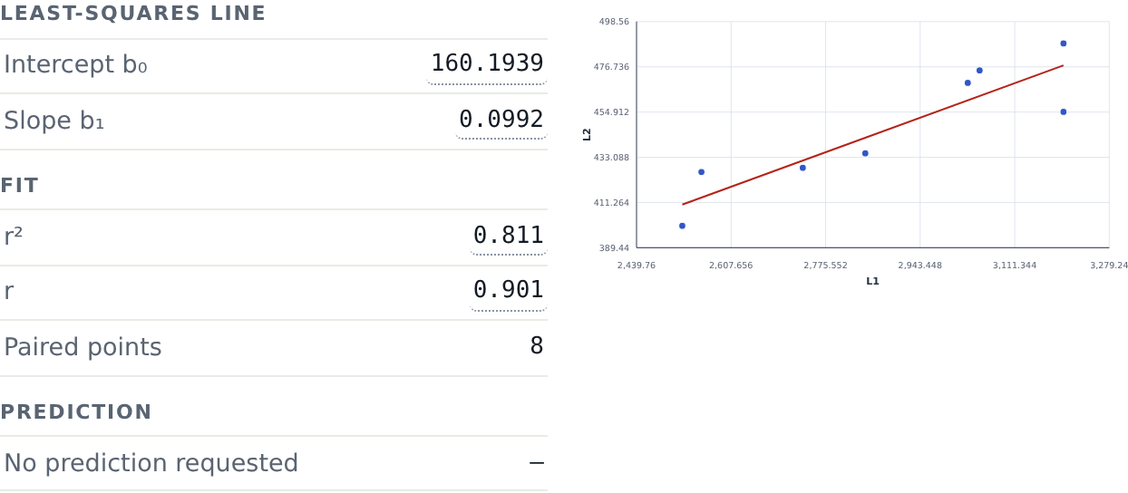
Reading the Regression Output
Running LinReg(a+bx) reports the least-squares regression line, its intercept and slope, and .
 Example
Predicting a Value
To predict the selling price of a house of a given size, substitute the size for x in the least-squares regression line.
A house of 2900 square feet is predicted to sell for about 447.9 thousand dollars.
Interpreting the Regression Coefficients
For a given value of x, the predicted value estimates the average y-value for all individuals with that x-value.
For a house of 2900 square feet, = 447.9 estimates the average price of all houses that size — not the price of any one house.
The y-intercept, , is the point where the line crosses the y-axis. This has a practical interpretation only when the data contain both positive and negative values of x.
Interpreting the Regression Coefficients
If the x-values of two points on a line differ by 1, their y-values will differ by an amount equal to the slope of the line. For example, if a line has a slope of 4, then two points whose x-values differ by 1 will have y-values that differ by 4. This enables us to interpret the slope . If the values of the explanatory variable differ by 1, their predicted values will differ by .
If the values of the explanatory variable differ by some other amount, say , their predicted values will differ by .
Here = 0.0992 thousand dollars per square foot — about $99 for every extra square foot.
House A is 2700 square feet — predicted price 428.0.
House B is 2850 square feet — predicted price 442.9.
The long way 442.9 − 428.0 = 14.9
The short way the sizes differ by 150, so (0.0992)(150) = 14.9
Two routes, one answer. Once you have the slope, you never needed the two predictions.
The long way 442.9 − 428.0 = 14.9
The short way the sizes differ by 150, so (0.0992)(150) = 14.9
Think About ItDo Not Extrapolate
The sizes in the data run from 2521 to 3198 square feet. The regression line describes that range. It says nothing about houses outside it.
Outside the data. No house this size was observed, so this prediction rests on nothing.
Inside the range of the data, the prediction is supported by the houses around it.
 Check Your Understanding
At the final exam in a class, the professor asks each student to indicate how many hours they studied for the exam. After grading the exam, the professor computes the least-squares regression line for predicting the final exam score from the number of hours studied. The equation of the line is .
Antoine studies for 6 hours. What is the expected exam score?
Emma studied for 3 hours longer than Jeremy did. How much higher is Emma’s score predicted to be?