MATH 1401 · Dr. Barry Monk

Random Variables

Section 6.1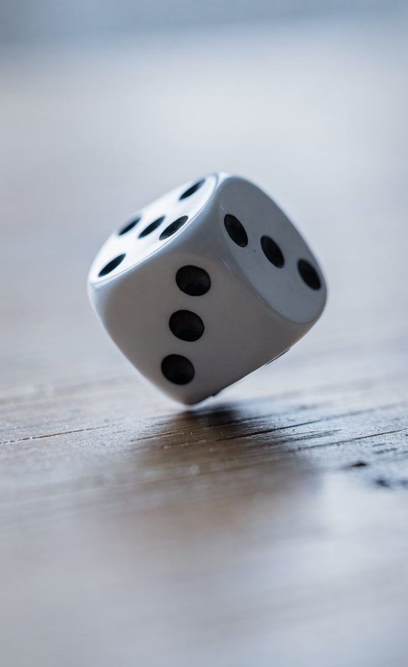

A white die with black pips tumbling across a wooden surface, caught mid-roll.

Definition

Random Variables

If we roll a fair die, the possible outcomes are the numbers 1, 2, 3, 4, 5, and 6.

Each of these numbers has probability $1 / 6$ . Rolling a die is a probability experiment whose outcomes are numbers. The outcome of such an experiment is called a random variable.

A random variable is a numerical outcome of a probability experiment.

Two large silver coins in raking light against a dark background, one turned to show an eagle.

Definition

Probability Distribution

A probability distribution for a discrete random variable specifies the probability for each possible value of the random variable.

Properties

0 \leq P (x) \leq 1

for every possible

x

\sum P (x) = 1

A hand flipping a quarter above a second, open hand, against a dark background.

Example

Example: Determining a Probability Distribution

A fair coin is tossed twice. Let $X$ be the number of heads that come up. Find the probability distribution of $X$ .

Solution:

There are four equally likely outcomes

First Toss	Second Toss	$X = Number of Heads$
H	H	2
H	T	1
T	H	1
T	T	0

There are three possible values for the number of heads ( $X$ ): 0, 1, and 2. One of the four outcomes has a value of “0”, two have the value “1”, and one has the value “2”. Therefore,

P (0) = \frac{1}{4} = 0.25,

P (1) = \frac{2}{4} = \frac{1}{2} = 0.50,

and

P (2) = \frac{1}{4} = 0.25 .

The probability distribution is

$x$	0	1	2
$P (x)$	0.25	0.50	0.25

Example

Example: Probability Distribution

Decide whether each of the following represents a probability distribution.

$x$	$P (x)$
1	0.25
2	0.65
3	−0.30
4	0.11

This is not a probability distribution because $P (3)$ is not between 0 and 1.

$x$	$P (x)$
−1	0.17
−0.5	0.25
0	0.31
0.5	0.22
1	0.05

This is a probability distribution. All probabilities are between 0 and 1 and they sum to 1.

$x$	$P (x)$
1	1.02
10	0.31
100	0.90
1000	0.43

This is not a probability distribution because $P (1)$ is not between 0 and 1.

Example

Example: Computing Probabilities

Four patients have made appointments to have their blood pressure checked at a clinic. Let $X$ be the number of them that have high blood pressure. The probability distribution of $X$ is as follows.

$x$	0	1	2	3	4
$P (x)$	0.23	0.41	0.27	0.08	0.01

a) Find $P (2 or 3)$

Solution:

We find the probability to be:

P (2 or 3) = P (2) + P (3) = 0.27 + 0.08 = 0.35

A clinician in a white coat presses a stethoscope to a patient’s inner elbow while a blood-pressure cuff is inflated on the upper arm.

Example

Example: Computing Probabilities

Four patients have made appointments to have their blood pressure checked at a clinic. Let $X$ be the number of them that have high blood pressure. The probability distribution of $X$ is as follows.

$x$	0	1	2	3	4
$P (x)$	0.23	0.41	0.27	0.08	0.01

b) Find $P (More than 1)$

Solution:

“More than 1” means “2 or 3 or 4.”

P (More than 1) = P (2 or 3 or 4) = 0.27 + 0.08 + 0.01 = 0.36

Example

Example: Computing Probabilities

Four patients have made appointments to have their blood pressure checked at a clinic. Let $X$ be the number of them that have high blood pressure. The probability distribution of $X$ is as follows.

$x$	0	1	2	3	4
$P (x)$	0.23	0.41	0.27	0.08	0.01

c) Find $P (At least 1)$

Solution:

The complement of “At least one” is “none”:

P (At least one) = 1 - P (0) = 1 - 0.23 = 0.77

Example

Example: Connection with Populations

An aerial view of a parking lot. Rows of cars sit under blue-roofed canopies on one side and in open bays on the other, with directional arrows painted on the asphalt.

A parking facility contains 1000 parking spaces categorized as follows.

Type of Space	Covered Long-Term	Covered Short-Term	Uncovered Long-Term	Uncovered Short-Term
Cost	$2.00	$4.50	$1.50	$4.00
Number of Spaces	142	378	423	57

A parking space is selected at random. Let $X$ represent the hourly parking fee for the randomly sampled space. Find the probability distribution of $X$ .

To find the probability distribution, we must list the possible values of $X$ and then find the probability of each of them. The possible values of $X$ are 1.50, 2.00, 4.00, 4.50. Next, we find their probabilities.

P (1.50) = \frac{# costing $1.50}{total # of spaces} = \frac{423}{1000} = 0.423

P (2.00) = \frac{# costing $2.00}{total # of spaces} = \frac{142}{1000} = 0.142

P (4.00) = \frac{# costing $4.00}{total # of spaces} = \frac{57}{1000} = 0.057

P (4.50) = \frac{# costing $4.50}{total # of spaces} = \frac{378}{1000} = 0.378

Probability Distribution

$x$	$P (x)$
1.50	0.423
2.00	0.142
4.00	0.057
4.50	0.378

Three clipboards laid on a pale surface, each holding a printed sheet headed Measurement Results with columns of trial numbers and values.

$\bar{x}$ is a Random Variable

Often when we draw a sample, we compute the sample mean $\bar{x}$ .

The quantity $\bar{x}$ is a random variable, because its value is different for different samples.

The probability distribution for $\bar{x}$ is usually difficult to compute. We will learn a way to approximate the probability distribution of the sample mean when the sample size is large in a later chapter.

Probability Histograms

Probability distributions can be represented with histograms to visualize the distribution.

Example:

The following presents the probability distribution and histogram for the number of heads in a sequence of five tosses, using the assumption that heads and tails are equally likely, and the tosses are independent events.

$x$	$P (x)$
0	0.03125
1	0.15625
2	0.31250
3	0.31250
4	0.15625
5	0.03125

The polished metal beam and central pivot of a balance scale, its two pans hanging level.

Definition

Mean of a Random Variable

The mean is a measure of center, and for a random variable, it represents the center of its probability distribution. The mean of a random variable is also called the expected value. To find the mean of a discrete random variable, multiply each possible value by its probability and sum the results.

Mean of a Random Variable (Expected Value)

μ_{X} = \sum [x \cdot P (x)]

Example

Example: Mean of a Random Variable

A computer monitor is composed of a large number of points of light called pixels. It is not uncommon for a few pixels to be defective. Let $X$ represent the number of defective pixels on a randomly chosen monitor. The probability distribution of $X$ is as follows. Find the mean number of defective pixels.

$x$	$P (x)$
0	0.2
1	0.5
2	0.2
3	0.1

The mean is

μ_{X} = (0) (0.2) + (1) (0.5) + (2) (0.2) + (3) (0.1) = 1.2 .

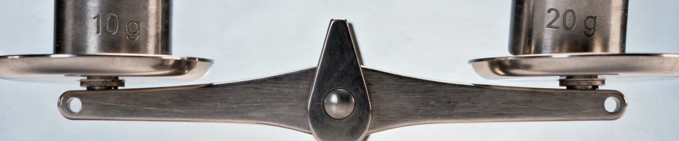
If we imagine each rectangle in the probability histogram to be a weight, the mean is the point at which the histogram would balance.

μ_{X} = 1.2

A young man in a jacket stands with folded arms beside a car at dusk, city lights behind him.

Expected Value

There are many occasions on which people want to predict how much they are likely to gain or lose if they make a certain decision or take a certain action. Often, this is done by computing the mean of a random variable.

In such situations, the mean is sometimes called the “expected value” and is denoted by $E (X)$ . If the expected value is positive, it is an expected gain, and if it is negative, it is an expected loss.

An aerial view of an oil field at dusk, a pump jack in the foreground and access roads and well pads running to the horizon.

Example

Example 1: Expected Value

A mineral economist estimated that a particular venture had probability 0.4 of a $30 million loss, probability 0.5 of a $20 million profit, and probability 0.1 of a $40 million profit. Let $X$ represent the profit. Find the probability distribution of the profit and the expected value of the profit. Does this venture represent an expected gain or an expected loss?

Solution:

The probability distribution is as follows. Note that 30 is negative since it represents a loss.

$x$	$P (x)$
−30	0.4
20	0.5
40	0.1

E (X) = (- 30) (0.4) + (20) (0.5) + (40) (0.1) = 2.0

There is an expected gain of $2 million.

Example

Example 2: Expected Value

An insurance company sells a one-year term life insurance policy to a 70-year-old man. The man pays a premium of $400. If he dies within one year, the company will pay $10,000 to his beneficiary. The probability that a 70-year-old man is still alive one year later is 0.9715. Let $X$ be the profit made by the insurance company. Find the expected value of the profit.

Solution:

If the man lives, the company keeps $400. If the man dies, the insurance company keeps $400, but has to pay $10,000, so its profit is −$9600.

The expected value is

E (X) = (- 9600) (0.0285) + (400) (0.9715) = 115

The expected gain for the insurance company is $115. We interpret this by saying that if the company sells many policies, it can expect to earn $115 for each policy on the average.

An older couple sit outdoors together, both smiling; the woman holds a tablet.

$x$	$P (x)$
−9600	0.0285
400	0.9715

1 / 23 → ← advance · Z zoom · B blank · H hides this bar

Random Variables

Random Variables

Distinguish between discrete and continuous random variables

Discrete and Continuous

Determine a probability distribution for a discrete random variable

Probability Distribution

Example: Determining a Probability Distribution

Example: Probability Distribution

Example: Computing Probabilities

Example: Computing Probabilities

Example: Computing Probabilities

Describe the connection between probability distributions and populations

Example: Connection with Populations

$\bar{x}$ is a Random Variable

Construct a probability histogram for a discrete random variable

Probability Histograms

Compute the mean of a discrete random variable

Mean of a Random Variable

Example: Mean of a Random Variable

Expected Value

Example 1: Expected Value

Example 2: Expected Value

Oversold

6.1 HW: Random Variables

Random Variables

Random Variables

Distinguish between discrete and continuous random variables

Discrete and Continuous

Determine a probability distribution for a discrete random variable

Probability Distribution

Example: Determining a Probability Distribution

Example: Probability Distribution

Example: Computing Probabilities

Example: Computing Probabilities

Example: Computing Probabilities

Describe the connection between probability distributions and populations

Example: Connection with Populations

x¯ is a Random Variable

Construct a probability histogram for a discrete random variable

Probability Histograms

Compute the mean of a discrete random variable

Mean of a Random Variable

Example: Mean of a Random Variable

Expected Value

Example 1: Expected Value

Example 2: Expected Value

Oversold

6.1 HW: Random Variables

$\bar{x}$ is a Random Variable