The Central Limit Theorem for Proportions & Assessing Normality

Sections 7.4 & 7.6

Today's Plan

You can already:

Find probabilities with a normal distribution

Find a value from a normal distribution with a given percentile

Find probabilities involving a sample mean using the Central Limit Theorem

Today:

Use the Central Limit Theorem for a sample proportion, $\hat{p}$

Find probabilities for a sample proportion

Use a dotplot to decide whether a sample came from an approximately normal population

Example

Review Problem: Hours of Sleep

Adults sleep an average of $μ = 6.8$ hours per night with standard deviation $σ = 1.4$ hours. Assume sleep times are normally distributed.

Question A: What is the probability that a randomly selected adult sleeps more than 7.5 hours?

Question B: A researcher samples 35 adults. What is the probability that the sample mean sleep time is more than 7.5 hours?

Think first

Both questions use the same cutoff, 7.5 hours. One is about one adult, the other is about the mean of 35 adults. Which standard deviation does each one use? And which probability will be smaller, by a little or by a lot?

A young man asleep on a sofa under a knitted blanket.

Example

Review Problem: Question A

What is the probability that a randomly selected adult sleeps more than 7.5 hours?

Recall

$μ = 6.8$ hours

$σ = 1.4$ hours

Solution:

One adult's sleep time is normally distributed with $μ = 6.8$ and $σ = 1.4$ .

Find the area under the normal curve:

Statistics Calculator

TI-84 Plus A TI-84 Plus home screen showing normalcdf(7.5,99999999,6.8,1.4) and its result, 0.3085375322.

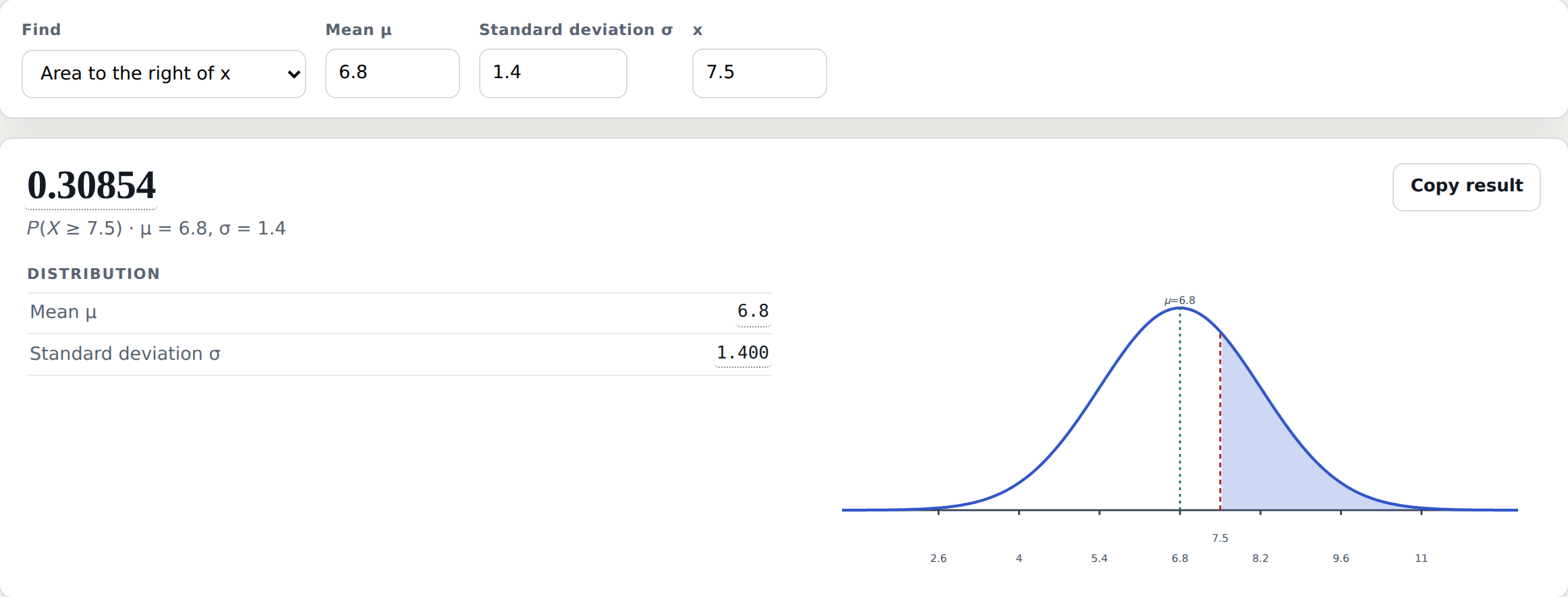
The probability that a randomly selected adult sleeps more than 7.5 hours is approximately 0.3085.

Example

Review Problem: Question B

A researcher samples 35 adults. What is the probability that the sample mean sleep time is more than 7.5 hours?

Recall

$μ = 6.8$ hours

$σ = 1.4$ hours

$n = 35$

Solution:

Since $n = 35 > 30$ , we can apply the Central Limit Theorem.

Compute $μ_{\bar{x}}$ and the standard error $σ_{\bar{x}}$ :

μ_{\bar{x}} = μ = 6.8

and

σ_{\bar{x}} = \frac{σ}{\sqrt{n}} = \frac{1.4}{\sqrt{35}} = 0.237

Find the area under the normal curve:

Statistics Calculator

TI-84 Plus A TI-84 Plus home screen showing normalcdf(7.5,99999999,6.8,0.237) and its result, 0.0015705914.

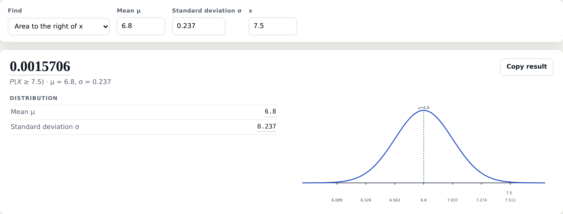
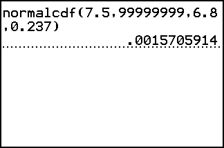
The probability that the sample mean sleep time is more than 7.5 hours is approximately 0.0016.

The Key Difference

Individual Adult

High variability: $σ = 1.4$ hours

Probability one adult sleeps more than 7.5 hours: $P (X > 7.5) = 0.3085$

Individual values are naturally spread out across the population

Sample of 35 Adults

Low variability: $σ_{\bar{x}} = \frac{1.4}{\sqrt{35}} = 0.237$ hours

Probability the sample mean of 35 adults is more than 7.5 hours: $P (\bar{x} > 7.5) = 0.0016$

Sample means cluster tightly around the population mean

Proportions: A Different Kind of Question

MEANS (

\bar{x}

)

Average hours of sleep

A teenager looking at a phone at a table.

Average time on TikTok

A white delivery van parked at the curb, with a hand truck and a cardboard box beside it.

Average delivery time

PROPORTIONS (

\hat{p}

)

Proportion of people who sleep less than 6 hours

Proportion of teenagers who use TikTok daily

Proportion of on-time deliveries

In a population, the proportion who have a certain characteristic is called the population proportion, denoted $p$ . In a simple random sample of $n$ individuals, if $x$ of them have the characteristic, the sample proportion is $\hat{p} = \frac{x}{n}$ .

Sampling Distribution of $\hat{p}$

Just as different samples produce different values of $\bar{x}$ . . .

. . . different samples will also produce different values of the sample proportion $\hat{p}$ .

Each sample: 1,000 people. 672 have the characteristic, so $\hat{p} = \frac{672}{1,000} = 0.672$

Because $\hat{p}$ varies from sample to sample, it has a probability distribution of its own, called the sampling distribution of $\hat{p}$ .

What Does the Sampling Distribution of $\hat{p}$ Look Like?

Population: 57% of people can correctly identify a deepfake video, so $p = 0.57$ ; 43% can't

Sample size $n = 80$

Think first

Before you draw, predict where the sample proportions will center and what shape they will make.

Samples0

Mean of the sample proportions

Standard deviation of the sample proportions

Draw more samples

The sample proportions pile up in the shape of a normal curve.

The Central Limit Theorem for MeansProportions

RECALL

$\bar{x}$ $\hat{p}$ is approximately normal with mean $μ_{\bar{x}} = μ$ $μ_{\hat{p}} = p$
and standard error $σ_{\bar{x}} = \frac{σ}{\sqrt{n}}$ $σ_{\hat{p}} = \sqrt{\frac{p (1 - p)}{n}}$ as long as
$n > 30$ or the population is approximately normal $n \cdot p$ and $n \cdot (1 - p)$ are both at least 10

Checking the Theorem Against the Machine

The machine drew samples of $n = 80$ from a population with $p = 0.57$ .

Theorem

μ_{\hat{p}}

0.57

Mean of the sample proportions

Theorem

σ_{\hat{p}}

0.0554

Standard deviation of the sample proportions

Center. The theorem says $μ_{\hat{p}} = p = 0.57$ .

Spread. The theorem says the standard error is $σ_{\hat{p}} = \sqrt{\frac{p (1 - p)}{n}} = \sqrt{\frac{0.57 (0.43)}{80}} = 0.0554$ .

Shape. The theorem says approximately normal, since $n \cdot p = 80 (0.57) = 45.6$ and $n \cdot (1 - p) = 80 (0.43) = 34.4$ are both at least 10. The machine's sample proportions piled up in the shape of a normal curve.

The theorem and the machine agree on all three.

Why Both Conditions Matter

1. Drag $n$ to the right until both conditions are met.

2. Leave $n$ there, and move $p$ close to 0 or close to 1.

3. Bring $p$ back to the middle, then lower $n$ .

When $p$ is close to 0 or close to 1, $n$ has to be larger. When $n$ is small, $p$ has to be near the middle.

Check your understanding

Does the Central Limit Theorem Apply?

Think first

For each one, compute $n \cdot p$ and $n \cdot (1 - p)$ .

(a)A simple random sample of size 60 will be drawn from a population with proportion $p = 0.12$ .

(a)NO. $n \cdot p = 60 (0.12) = 7.2$ , which is less than 10.

(b)A simple random sample of size 24 will be drawn from a population with proportion $p = 0.55$ .

(b)YES. $n \cdot p = 24 (0.55) = 13.2$ and $n \cdot (1 - p) = 24 (0.45) = 10.8$ are both at least 10.

(c)A simple random sample of size 10,000 will be drawn from a population with proportion $p = 0.002$ .

(c)YES. $n \cdot p = 10,000 (0.002) = 20$ and $n \cdot (1 - p) = 10,000 (0.998) = 9,980$ are both at least 10.

Computing Probabilities for $\hat{p}$

Check that $n \cdot p \geq 10$ and $n \cdot (1 - p) \geq 10$

Find $μ_{\hat{p}} = p$ and the standard error $σ_{\hat{p}} = \sqrt{\frac{p (1 - p)}{n}}$

Same normal curve work as for sample means: find the area under the normal curve

Example

Example 1: Deepfake Detection

A 2024 meta-analysis of 56 studies found that only 57% of people can correctly identify a deepfake video. A media literacy organization tests 80 people. What is the probability that fewer than half correctly identify the deepfake?

Solution:

We have $n = 80$ and $p = 0.57$

$n \cdot p = 80 (0.57) = 45.6$ ✓

$n \cdot (1 - p) = 80 (0.43) = 34.4$ ✓

A man in glasses studies a woman's face on a computer monitor.

Example

Example 1: Deepfake Detection

What is the probability that fewer than half correctly identify the deepfake?

Recall

$n = 80$

$p = 0.57$

Compute:

μ_{\hat{p}} = p = 0.57

and

σ_{\hat{p}} = \sqrt{\frac{p (1 - p)}{n}} = \sqrt{\frac{0.57 (0.43)}{80}} = 0.0554

Find the area under the normal curve:

Statistics Calculator

TI-84 Plus A TI-84 Plus home screen showing normalcdf(-99999,0.5,0.57,0.0554) and its result, 0.103198032.

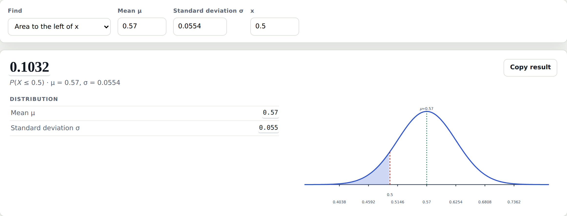
The probability that fewer than half correctly identify the deepfake is approximately 0.1032.

Example

Example 2: Bike Lane Support

A 2019 city study found that 49% of residents supported adding bike lanes. You believe support has grown since then. You survey 200 residents and find 55% now support it. If support hasn't changed, what is the probability of getting a sample proportion at least this high?

Solution:

We have $n = 200$ and $p = 0.49$

$n \cdot p = 200 (0.49) = 98$ ✓

$n \cdot (1 - p) = 200 (0.51) = 102$ ✓

Two cyclists in helmets riding in a painted bike lane on a city street.

Example

Example 2: Bike Lane Support

If support hasn't changed, what is the probability of getting a sample proportion at least this high?

Recall

$n = 200$

$p = 0.49$

Compute:

μ_{\hat{p}} = p = 0.49

and

σ_{\hat{p}} = \sqrt{\frac{p (1 - p)}{n}} = \sqrt{\frac{0.49 (0.51)}{200}} = 0.0353

The standard error uses $p = 0.49$ , the value we're assuming, not the sample's $\hat{p} = 0.55$ .

Find the area under the normal curve:

Statistics Calculator

TI-84 Plus A TI-84 Plus home screen showing normalcdf(0.55,9999,0.49,0.0353) and its result, 0.044592081.

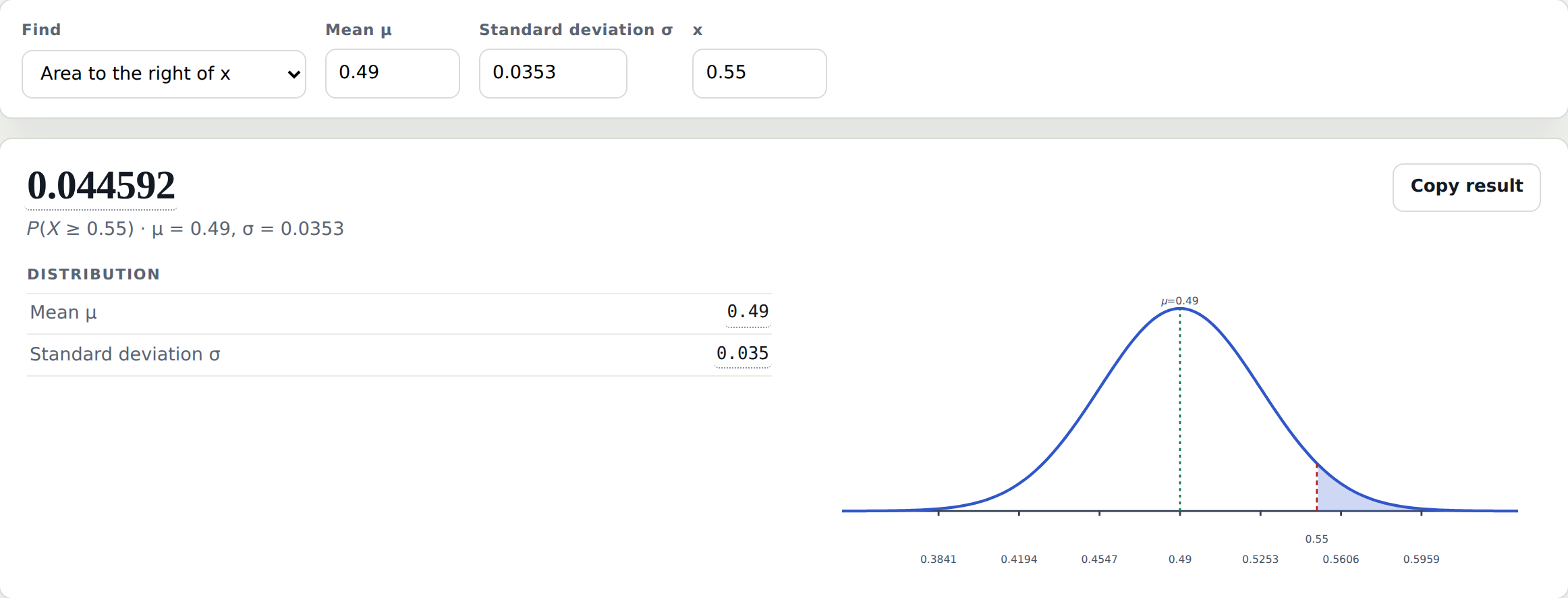
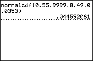
If support hasn't changed, the probability of a sample proportion of 0.55 or more is approximately 0.0446.

Unusual? 0.0446 is less than 0.05, so if support hasn't changed, a sample proportion this high would be unusual.

Example

Example 3: Who Wants Ice Cream!

A Harris poll found that 27% of Americans prefer chocolate ice cream. A food blogger thinks Gen Z prefers chocolate more than the general population. She surveys 100 college students and finds 30% prefer chocolate. What is the probability of getting a sample proportion at least this high if Gen Z is the same as everyone else?

Solution:

We have $n = 100$ and $p = 0.27$

$n \cdot p = 100 (0.27) = 27$ ✓

$n \cdot (1 - p) = 100 (0.73) = 73$ ✓

Three ice cream cones in a row, a chocolate scoop with fudge sauce in front.

Example

Example 3: Who Wants Ice Cream!

What is the probability of getting a sample proportion at least this high if Gen Z is the same as everyone else?

Recall

$n = 100$

$p = 0.27$

Compute:

μ_{\hat{p}} = p = 0.27

and

σ_{\hat{p}} = \sqrt{\frac{p (1 - p)}{n}} = \sqrt{\frac{0.27 (0.73)}{100}} = 0.0444

Find the area under the normal curve:

Statistics Calculator

TI-84 Plus A TI-84 Plus home screen showing normalcdf(0.30,9999,0.27,0.0444) and its result, 0.2496232196.

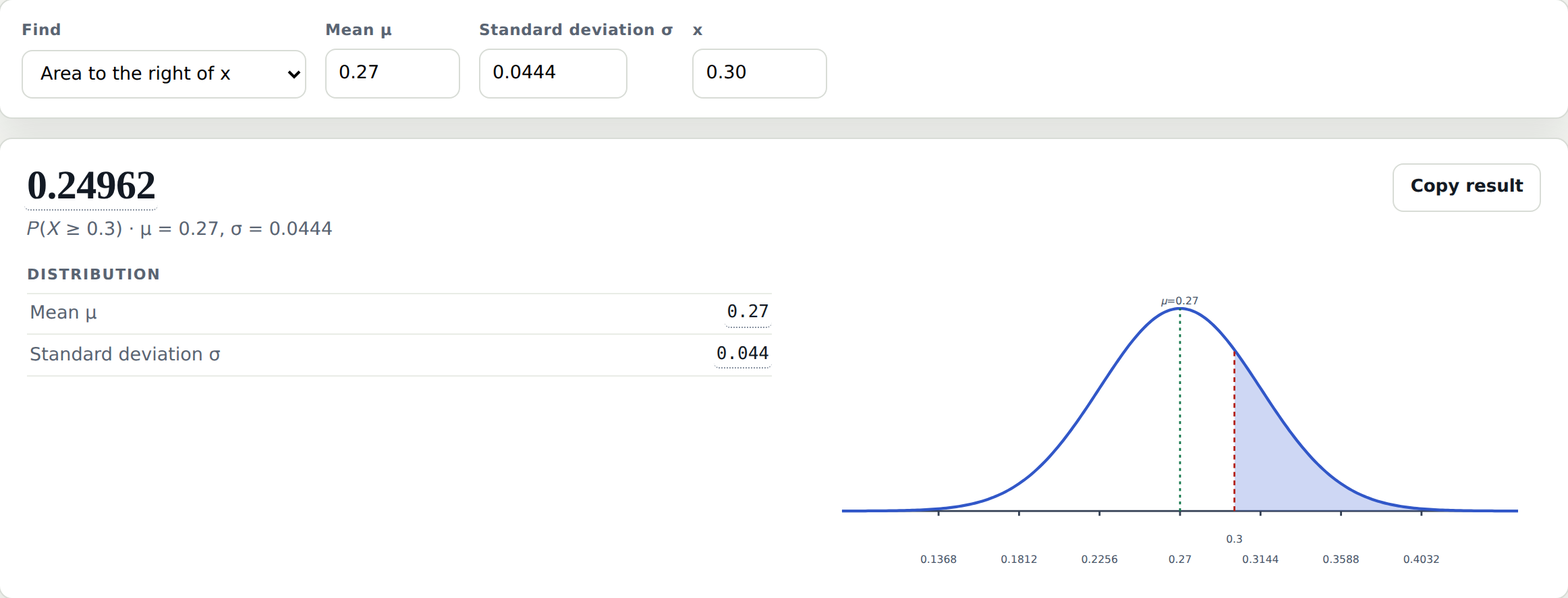
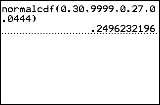
If Gen Z is the same as everyone else, the probability of a sample proportion of 0.30 or more is approximately 0.2496.

Unusual? 0.2496 is not less than 0.05, so if Gen Z is the same as everyone else, a sample proportion this high would not be unusual.

You Are Ready For:

7.4 & 7.6: Central Limit Theorem for Proportions & Assessing Normality

Check that $n \cdot p$ and $n \cdot (1 - p)$ are both at least 10

Find the mean of $\hat{p}$ and its standard error: $p$ and $\sqrt{\frac{p (1 - p)}{n}}$

Find probabilities for a sample proportion

Use a dotplot to check a sample for outliers, severe skewness and multiple modes

1 / 28 → ← advance · Z zoom · B blank · H hides this bar

The Central Limit Theorem for Proportions & Assessing Normality

Today's Plan

Review Problem: Hours of Sleep

Review Problem: Question A

Review Problem: Question B

The Key Difference

Has Support Grown?

Proportions: A Different Kind of Question

Sampling Distribution of $\hat{p}$

What Does the Sampling Distribution of $\hat{p}$ Look Like?

The Central Limit Theorem for MeansProportions

Checking the Theorem Against the Machine

Why Both Conditions Matter

Does the Central Limit Theorem Apply?

Computing Probabilities for $\hat{p}$

Example 1: Deepfake Detection

Example 1: Deepfake Detection

Example 2: Bike Lane Support

Example 2: Bike Lane Support

Example 3: Who Wants Ice Cream!

Example 3: Who Wants Ice Cream!

Assessing Normality

When We Reject Normality

Example 4: Oven Temperatures

Example 5: Heart Rate Monitoring

Approximately Normal or Not?

You Are Ready For:

The Central Limit Theorem for Proportions & Assessing Normality

Today's Plan

Review Problem: Hours of Sleep

Review Problem: Question A

Review Problem: Question B

The Key Difference

Has Support Grown?

Proportions: A Different Kind of Question

Sampling Distribution of p^

What Does the Sampling Distribution of p^ Look Like?

The Central Limit Theorem for MeansProportions

Checking the Theorem Against the Machine

Why Both Conditions Matter

Does the Central Limit Theorem Apply?

Computing Probabilities for p^

Example 1: Deepfake Detection

Example 1: Deepfake Detection

Example 2: Bike Lane Support

Example 2: Bike Lane Support

Example 3: Who Wants Ice Cream!

Example 3: Who Wants Ice Cream!

Assessing Normality

When We Reject Normality

Example 4: Oven Temperatures

Example 5: Heart Rate Monitoring

Approximately Normal or Not?

You Are Ready For:

Sampling Distribution of $\hat{p}$

What Does the Sampling Distribution of $\hat{p}$ Look Like?

Computing Probabilities for $\hat{p}$