Confidence Intervals for a Population Mean ( Unknown)
Section 8.2The Structure of a Confidence Interval
Every confidence interval has the same basic structure:
Confidence Interval:
Confidence Interval:
What If We Don't Know ?
If we knew :
Confidence Interval:
Since we don't know :
Confidence Interval:
estimates , but varies from sample to sample
Extra uncertainty means the standard normal curve no longer gives the right critical value.
It comes from something called the Student's distribution.
What is a Distribution?
distributions are symmetric and unimodal, like the normal distribution, but more spread out.
Why the extra spread?
We are estimating with , which introduces uncertainty. To maintain the same confidence level, we need a wider interval. The distribution builds this in.
Why is there more than one?
Different sample sizes have different amounts of uncertainty. Each needs its own distribution.
We distinguish them by a quantity related to the sample size called degrees of freedom.
The number of degrees of freedom is .
1 Degree of Freedom
4 Degrees of Freedom
10 Degrees of Freedom
Degrees of Freedom
Degrees of freedom
Fewer degrees of freedom → more uncertainty → wider distribution
More degrees of freedom → is close to → nearly normal
What we'll do: drag the slider from 1 degree of freedom up to 30.
What to look for: how the dashed curve compares with the standard normal curve.
As the degrees of freedom increase, the curve gets closer to the standard normal curve.
- By 30 degrees of freedom, the two curves nearly coincide.
Degrees of freedom: 1
Drag the degrees-of-freedom slider from 1 up to 30.
Confidence Interval When Is Unknown
| Sample size | Degrees of freedom | |
|---|---|---|
| 5 | 4 | 2.776 |
| 10 | 9 | 2.262 |
| 30 | 29 | 2.045 |
| 100 | 99 | 1.984 |
| Standard normal, | 1.960 | |
is noticeably larger than when is small, but gets closer to it as grows.
Why Not Just Use ?
What we'll do: draw samples of 5 from a normal population with and , and build a 95% interval from each one two ways, with on the left and on the right.
What to look for: the percent of intervals in each column that contain .
In the long run, about 88% of the intervals contain , but about 95% of the intervals do.
- So when is unknown, we use .
Press Draw 50 twice.
Assumptions
When is known:
CLT → Sampling distribution of is normal
When is not known:
Same CLT conditions apply → Use
Caveat:
When the sample size is small, we must check whether the population can be assumed to be normal. Draw a dotplot and look for skewness or outliers.

 Example
 1: Grocery Delivery
Among 40 deliveries sampled by a grocery delivery service, the mean delivery time was 34.2 minutes with a standard deviation of 8.6 minutes. Construct a 95% confidence interval for the mean delivery time.
Check the assumptions:
Confidence level = 0.95
 Example
 1: Grocery Delivery


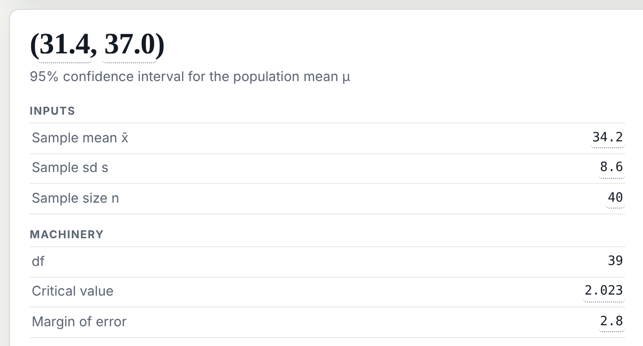 Example
 1: Grocery Delivery
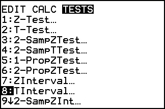
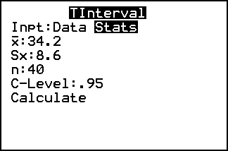
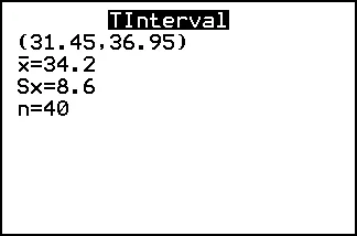
We are 95% confident that the mean delivery time is between 31.4 and 37.0 minutes.
ExampleExample 2: Hours of Sleep
Seven college students were randomly selected and asked how many hours of sleep they got last night. The results were 7.0, 8.5, 6.5, 7.0, 5.0, 8.0, 6.0. Construct a 90% confidence interval for the mean hours of sleep.
Check the assumptions:
A dotplot reveals no outliers or strong skewness. It is reasonable to assume the population is normal. ✓
 Example
 2: Hours of Sleep
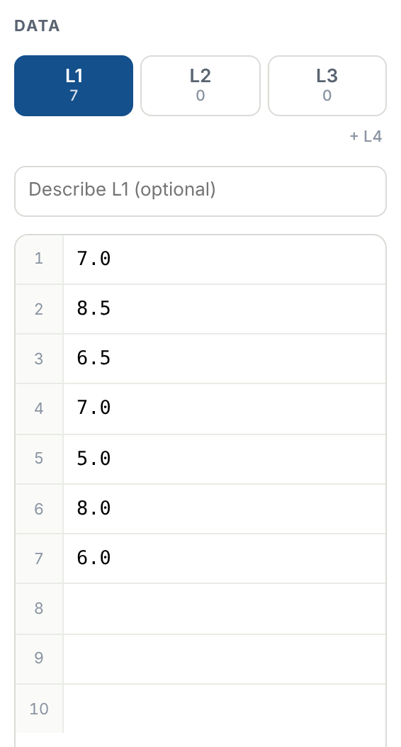

7.0, 8.5, 6.5, 7.0, 5.0, 8.0, 6.0
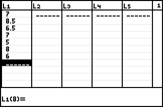
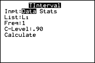
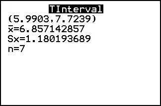
We are 90% confident that the mean sleep time is between 5.99 and 7.72 hours.
ExampleExample 3: Electric Vehicle Range
An electric vehicle manufacturer claims that its newest model has a mean driving range of 310 miles on a full charge. A consumer advocacy group tested 70 randomly selected vehicles and found a mean range of 298.4 miles with a standard deviation of 24.1 miles. Construct a 95% confidence interval for the mean range. Does the interval contradict the manufacturer's claim?
 Example
 3: Electric Vehicle Range
Construct a 95% confidence interval for the mean range. Does the interval contradict the manufacturer's claim?
claim: 310 miles
, ,

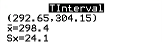
We are 95% confident that the mean driving range is between 292.7 and 304.1 miles.
Because 310 is not in the interval, the confidence interval does contradict the manufacturer's claim.
ExampleExample 4: Emergency Room Wait Times
A hospital claims that the mean wait time in its emergency room is less than an hour. A patient advocacy group surveyed 100 randomly selected patients and found a mean wait time of 54.2 minutes with a standard deviation of 17.6 minutes. Construct a 90% confidence interval. Does the interval contradict the hospital's claim?
 Example
 4: Emergency Room Wait Times
Construct a 90% confidence interval. Does the interval contradict the hospital's claim?
claim: less than 60 minutes
, ,

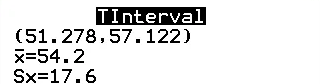
We are 90% confident that the mean waiting time is between 51.3 and 57.1 minutes.
Because all values in the confidence interval are less than one hour (60 minutes), the confidence interval does not contradict the hospital's claim.
ExampleExample 5: Coffee Shop Tips
A coffee shop owner wants to estimate the mean tip amount for a given day. A random sample of 9 tips yielded the following amounts (in dollars):
0.750.251.000.820.801.5010.000.501.50
Construct a 95% confidence interval for the mean tip amount.
Check the assumptions:
A dotplot reveals an outlier and strong skewness.
It is not reasonable to assume the population is normal. ✗

 Check your understanding
Can We Use This Method?
For each situation, is unknown. Can we construct a confidence interval for using the methods of this section?
(a)A simple random sample of 12, from a population that is approximately normal
(a)Yes
(b)A simple random sample of 18, whose dotplot shows an outlier
(b)No
(c)A simple random sample of 75, from a population that is skewed
(c)Yes
(d)200 people who chose to answer an online poll
(d)No: a voluntary response sample
Case StudyA Real-World Case
The Question:
Among people hospitalized with COVID-19, do vaccinated patients have better outcomes than unvaccinated patients?
The Data:
| Group | Sample Size |
|---|---|
| Vaccinated | 7,847 |
| Unvaccinated | 21,525 |
Source: Lee et al. (2023), 180+ hospitals, January to December 2021
 Case Study
A Real-World Case
What Was Measured:
The Findings:
| Group | Mean | 95% CI |
|---|---|---|
| Vaccinated | 8.04 days | (7.84, 8.24) |
| Unvaccinated | 9.49 days | (9.34, 9.64) |
| Group | Proportion | 95% CI |
|---|---|---|
| Vaccinated | 0.216 | (0.207, 0.225) |
| Unvaccinated | 0.269 | (0.263, 0.275) |
Case StudyA Real-World Case
The confidence intervals do not overlap in either case.
Vaccinated Patients:
Keep in Mind:
This study only looked at patients already hospitalized. Vaccination also reduces the chance of infection, severe symptoms, and hospitalization in the first place.
Bottom Line:
By the numbers, there's very little doubt that vaccinated patients fared much better.
You Are Ready For:
8.2: Confidence Intervals for a Population Mean ( Unknown)
Describe the Student's distribution and its degrees of freedom
Check the assumptions, with a dotplot when the sample is small
Construct a confidence interval for with technology
Interpret it, and decide whether it contradicts a claim