Hypothesis Tests for Proportions and Means

Sections 9.3 & 9.4

Case Study

The 5-Second Rule

A campus health researcher suspects that college students are more likely than the general public to follow the 5-second rule. She surveys a random sample of 200 college students and finds that 102 of them believe in it.

The sample proportion is $\hat{p} = \frac{102}{200} = 0.51$ , which is higher than the national rate of 0.44. But is that difference large enough to draw a real conclusion, or could it simply be due to chance?

Case Study

Setting Up the Test

A young man kneels on one knee, barefoot, on a kitchen floor, eating a piece of food he has picked up off it, with crumbs scattered on the tiles in front of him.

To answer this question, we perform a hypothesis test.

The null hypothesis is that college students believe in the 5-second rule at the same rate as the general public:

$H_{0} : p = 0.44$

The alternate hypothesis represents the claim that college students are more likely to believe in it:

$H_{1} : p > 0.44$

We have a right-tailed test.

Case Study

The Logic of the Test

We assume the null hypothesis is true and ask: if $p$ really were 0.44, how likely would we be to observe a sample proportion as high as 0.51?

If that outcome would be very unlikely, we reject $H_{0}$ . If it's reasonably likely, we do not reject $H_{0}$ .

Before performing the test, we choose a significance level $α$ : the maximum probability of a Type I error we are willing to accept.

A Type I error means rejecting $H_{0}$ when it's actually true: concluding that college students are more likely to believe the 5-second rule when they actually are not.

We use $α = 0.05$ (the most common choice).

A woman in glasses sits at a wooden desk with a pen at her chin, reading a completed survey form, with a stack of surveys and a mug in front of her and bookshelves behind.

Case Study

The Test Statistic

If $H_{0}$ is true, $\hat{p}$ follows an approximately normal distribution with $μ_{\hat{p}} = p_{0} = 0.44$ and standard error: $σ_{\hat{p}} = \sqrt{\frac{0.44 (1 - 0.44)}{200}} = 0.0351$ .

We compute a quantity called the test statistic, which is the $z$ -score of $\hat{p} = 0.51$ : $z = \frac{\hat{p} - μ_{\hat{p}}}{σ_{\hat{p}}} = \frac{0.51 - 0.44}{0.0351} \approx 1.994$ .

The observed value $\hat{p} = 0.51$ is fairly far out in the tail of the distribution, well above the null hypothesis value $p = 0.44$ . Intuitively, the evidence against $H_{0}$ appears to be strong.

We need a way to measure precisely how far out $\hat{p} = 0.51$ really is.

Case Study

The $P$ -Value

The $P$ -value answers this question:

If $H_{0}$ were true, what is the probability of observing a test statistic as extreme as ours, or more extreme?

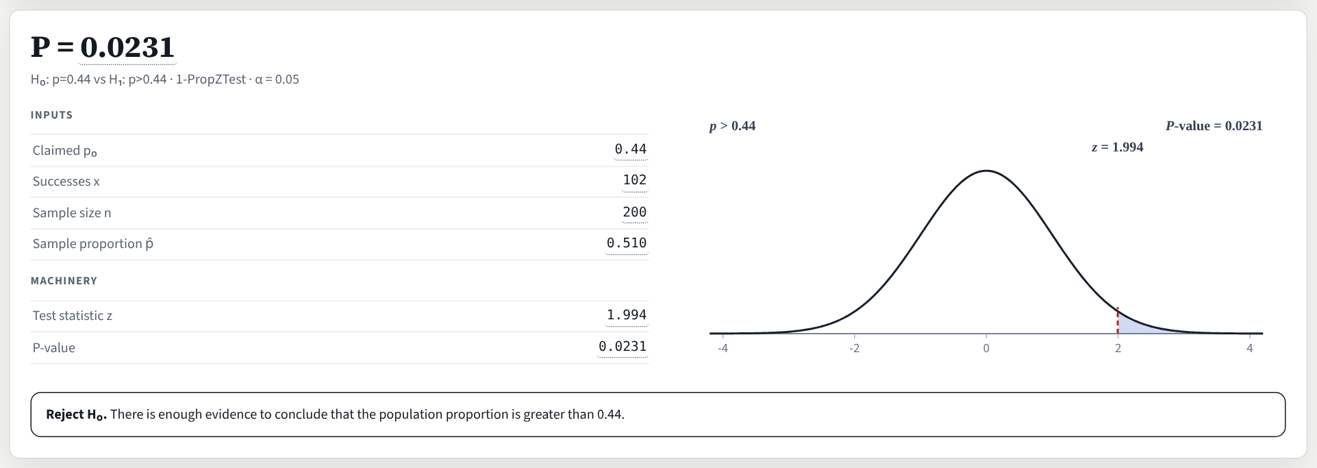
For a right-tailed test, the $P$ -value is the area to the right of $z = 1.994$ , which we find to be 0.0231. In other words, if the true proportion were 0.44, there's only about a 2.3% chance of getting a sample proportion as high as 0.51.

Watching the $P$ -Value Change

Curve: the standard normal curveShaded: the

P

-value

The plan

What we'll do: drag $z$ from 1.994 farther out to the right, then switch to a two-tailed test.

What to look for: the shaded area and the $P$ -value.

Try it

Drag $z$ out to 2.5.

The farther out the test statistic, the smaller the $P$ -value.

At $z = 2.50$ , the $P$ -value is 0.0062.
Two-tailed: both tails count, so the $P$ -value doubles, to 0.0124.

Try it

Press Two-tailed.

The $P$ -Value

The smaller the $P$ -value, the stronger the evidence against $H_{0}$ .

$P$ -value	Interpretation
Less than 0.01	Very strong evidence against $H_{0}$
0.01 to 0.05	Strong evidence against $H_{0}$
0.05 to 0.10	Moderate evidence against $H_{0}$
Greater than 0.10	Weak (or very little) evidence against $H_{0}$

QUESTION

How small does the $P$ -value have to be to reject $H_{0}$ ?

ANSWER

Less than or equal to the significance level $α$ .

RULE

If $P$ -value $\leq α$ → Reject $H_{0}$

Otherwise → Fail to reject $H_{0}$

Case Study

The 5-Second Rule

$H_{0} : p = 0.44$

$H_{1} : p > 0.44$

Because the $P$ -value (0.0231) is less than the level of significance (0.05), we reject $H_{0}$ .

There is sufficient evidence at the $α = 0.05$ level to conclude that college students are more likely than the general public to believe in the 5-second rule.

Check your understanding

Make the Decision

A city library reports that 30% of residents hold a library card. A librarian suspects the rate is higher, so she tests $H_{0} : p = 0.30$ vs. $H_{1} : p > 0.30$ . Her $P$ -value is 0.018.

(a)She tests at $α = 0.05$ . Does she reject $H_{0}$ ? State the conclusion.

0.018 \leq 0.05

, so she rejects

H_{0}

. There is sufficient evidence at the

α = 0.05

level to conclude that the proportion of residents who hold a library card is greater than 30%.

(b)She tests at $α = 0.01$ instead. Does she reject $H_{0}$ ? State the conclusion.

0.018 > 0.01

, so she does not reject

H_{0}

. There is not sufficient evidence at the

α = 0.01

level to conclude that the proportion of residents who hold a library card is greater than 30%.

Testing a Proportion with Technology

Statistics Calculator

The same form filled in: claimed p naught 0.44, successes x 102, sample size n 200, the alternate hypothesis set to greater than, right-tailed, and significance alpha 0.05.

The result: P = 0.0231. Claimed p naught 0.44, successes 102, sample size 200, sample proportion p-hat 0.510; test statistic z = 1.994 and P-value 0.0231; a normal curve with the area to the right of z = 1.994 shaded; and the verdict, Reject H naught: there is enough evidence to conclude that the population proportion is greater than 0.44.

Recall

$H_{0} : p = 0.44$

$H_{1} : p > 0.44$

$x = 102$

$n = 200$

$α = 0.05$

TI-84 Plus: 1-PropZTest

The 1-PropZTest command performs a hypothesis test for a population proportion. Access it by pressing STAT and choosing the TESTS menu.

The required inputs are $x$ and $n$ . If you know $\hat{p}$ instead, you can compute $x = \hat{p} \cdot n$ .

Assumptions

The following assumptions are the conditions under which the Central Limit Theorems let us use standard inference methods for proportions and means.

Testing a Population Proportion $p$	Testing a Population Mean $μ$
We have a simple random sample The population is at least 20 times as large as the sample. The values $n p_{0}$ and $n (1 - p_{0})$ are both at least 10.	We have a simple random sample The sample size is large $(n > 30)$ or the population is approximately normal.

Why Assumptions Matter

A checklist on a clipboard with seven boxes down the page, every one ticked except the third, which is marked with an X, and a pen lying beside it.

Assumptions aren't formalities, they are the conditions under which the math is valid.

When assumptions are violated:

$P$ -values become meaningless
Conclusions can't be trusted
Papers get retracted

Retraction Watch tracks scientific papers that have been withdrawn due to errors, fraud, or methodological problems, including statistical violations.

Example

Example 1: Defect Rate

Inspectors in hard hats, safety glasses and lab coats stand along a production line, checking trays of small bottles and noting results on clipboards.

A manufacturer guarantees that no more than 8% of its products are defective. After upgrading equipment, quality control runs a routine audit. In a random sample of 400 items, 24 are defective. Does the data support that the defect rate has dropped below 8%? Test at $α = 0.05$ .

Solution

$H_{0} : p = 0.08$ vs. $H_{1} : p < 0.08$

Check assumptions:

Simple random sample ✓
Reasonable to believe that the population is at least 20 times as large as the sample ✓
$n p_{0} = 400 \times 0.08 = 32 \geq 10$ ✓
$n (1 - p_{0}) = 400 \times 0.92 = 368 \geq 10$ ✓

Example

Example 1: Defect Rate

Recall

$n = 400$

$x = 24$

$H_{0} : p = 0.08$

$H_{1} : p < 0.08$

$α = 0.05$

In a left-tailed test, the $P$ -value is the area to the left of the test statistic.

Perform the test:

Statistics Calculator

TI-84 Plus

Because the $P$ -value is greater than $α$ , we do not reject $H_{0}$ .

There is not sufficient evidence to conclude that the defect rate has dropped below 8%.

Example

Example 2: Public Transit

A line of commuters in work clothes boards a city bus at a stop, with the driver at the wheel.

Before approving funding for modifying bus routes, a city council requires evidence that ridership has changed from the previous rate of 35%. A random sample of 250 residents finds that 30% commute by public transit. Use $α = 0.05$ level of significance.

Solution

$H_{0} : p = 0.35$ vs. $H_{1} : p \neq 0.35$

Check assumptions:

Simple random sample ✓
Reasonable to believe that the population is at least 20 times as large as the sample ✓
$n p_{0} = 250 \times 0.35 = 87.5 \geq 10$ ✓
$n (1 - p_{0}) = 250 \times 0.65 = 162.5 \geq 10$ ✓

Example

Example 2: Public Transit

$\hat{p} \times n = 0.30 \times 250 = 75$

Perform the test:

Statistics Calculator

TI-84 Plus

Recall

$n = 250$

$\hat{p} = 0.30$

$H_{0} : p = 0.35$

$H_{1} : p \neq 0.35$

$α = 0.05$

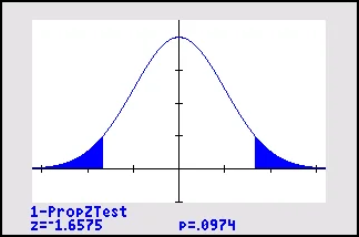
In a two-tailed test, the $P$ -value includes area from both tails: the probability of being this far from $p_{0}$ in either direction.

Because the $P$ -value is greater than $α$ , we do not reject $H_{0}$ .

There is not sufficient evidence to conclude that the proportion of residents who commute by public transit has changed from 35%.

Testing a Mean with Technology

When $σ$ is unknown, the test statistic for a mean is $t = \frac{\bar{x} - μ_{0}}{\frac{s}{\sqrt{n}}}$ .

If $H_{0}$ is true, it follows a Student's $t$ distribution with $n - 1$ degrees of freedom.

Statistics Calculator

The Hypothesis test tool set for a population mean: About a set to Population mean mu, One sample, population standard deviation sigma Unknown, from Summary statistics; claimed mu naught 75.6, sample mean x-bar 74.1, sample sd s 6.2, sample size n 36, the alternate hypothesis set to less than, left-tailed, and significance alpha 0.05.

The result: P = 0.0778. Claimed mu naught 75.6, sample mean x-bar 74.1, sample sd 6.2, sample size 36; test statistic t = −1.452 with 35 degrees of freedom, and P-value 0.0778; a curve with its left tail shaded; and the verdict, Fail to reject H naught: there is not enough evidence to conclude that the population mean is less than 75.6.

Givens

$H_{0} : μ = 75.6$

$H_{1} : μ < 75.6$

$\bar{x} = 74.1$

$s = 6.2$

$n = 36$

$α = 0.05$

TI-84 Plus: T-Test

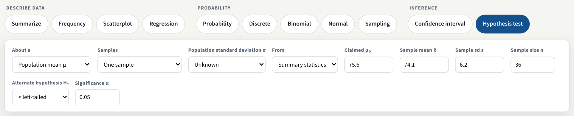
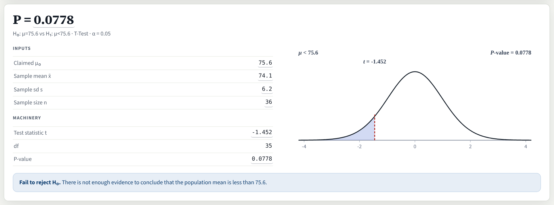
If we are testing a population mean, we use the T-Test command.

The required inputs are $\bar{x}$ , $s$ , and $n$ .

Example

Example 3: Battery Life

A smartphone manufacturer advertises 24-hour battery life. After complaints, the company runs a test. A random sample of 35 phones has a mean battery life of 22.1 hours with a standard deviation of 3.8 hours. Test whether the mean battery life is less than advertised. Use $α = 0.01$ level of significance.

Solution

$H_{0} : μ = 24$ vs. $H_{1} : μ < 24$

Check assumptions:

Simple random sample ✓
$n = 35 > 30$ ✓

A smartphone lies on a table beside a coiled charging cable, its screen showing a nearly empty battery icon.

Example

Example 3: Battery Life

Recall

$\bar{x} = 22.1$

$s = 3.8$

$n = 35$

$H_{0} : μ = 24$

$H_{1} : μ < 24$

$α = 0.01$

Perform the test:

Statistics Calculator

TI-84 Plus

Because the $P$ -value is less than $α$ , we reject $H_{0}$ .

There is sufficient evidence to conclude that the mean battery life is less than 24 hours.

The customer complaints appear to be justified.

Example

Example 4: Latte Calories

A large cup of latte topped with whipped cream sits on a saucer on a wooden coffee shop table, beside a small jar of syrup and a spoon.

A nutrition blogger suspects that a coffee chain's vanilla latte contains more than the advertised 250 calories. She collects a random sample of 18 lattes from various locations. The sample has a mean of 281 calories with a standard deviation of 64 calories. At the 0.05 significance level, is there evidence that the mean exceeds 250 calories?

Solution

$H_{0} : μ = 250$ vs. $H_{1} : μ > 250$

Check assumptions:

Simple random sample ✓
$n = 18 ≯ 30$ ✗

We have no information about the population to suggest it may be approximately normal.

We cannot justify performing the test.

The blogger would need to collect more data or provide evidence that calorie counts are approximately normally distributed.

Example

Example 5: A Generic Drug

Before a generic drug can be sold in the U.S., the FDA requires testing to confirm it performs equivalently to the brand-name version. A pharmaceutical company tests a generic topical pain reliever. The brand-name version delivers a mean of 3.5 micrograms of active ingredient per square centimeter of skin.

Seven volunteers apply the generic ointment. After six hours, the amount absorbed (in micrograms) is:

2.63.22.13.03.12.93.7

Is there evidence at the $α = 0.01$ level that the generic delivers a different amount?

A gloved technician squeezes ointment from a tube onto a square marked on a seated woman's forearm, as she watches.

Solution

$H_{0} : μ = 3.5$ vs. $H_{1} : μ \neq 3.5$

Check assumptions:

Simple random sample ✓
$n = 7$ → we must check for normality

There is no evidence of outliers or strong skewness,

so it is reasonable to assume the population is approximately normal.

Example

Example 5: A Generic Drug

Recall

2.6, 3.2, 2.1, 3.0, 3.1, 2.9, 3.7

$H_{0} : μ = 3.5$

$H_{1} : μ \neq 3.5$

$α = 0.01$

Perform the test:

Statistics Calculator

TI-84 Plus

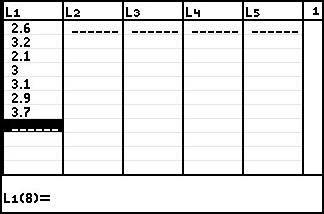
The $P$ -value is greater than $α$ , so we do not reject $H_{0}$ .

There is not sufficient evidence at the $α = 0.01$ level to conclude that the mean amount absorbed differs from 3.5 micrograms.

You Are Ready For:

Sections 9.3 & 9.4: Hypothesis Tests for Proportions and Means

Find the test statistic and the $P$ -value, and use the $P$ -value to decide whether to reject $H_{0}$

Check the assumptions before testing a population proportion or a population mean

Perform a test with technology, and state the conclusion in words

1 / 29 → ← advance · Z zoom · B blank · H hides this bar

Hypothesis Tests for Proportions and Means

The 5-Second Rule

The 5-Second Rule

Setting Up the Test

The Logic of the Test

The Test Statistic

The P-Value

Watching the P-Value Change

The P-Value

The 5-Second Rule

Make the Decision

Testing a Proportion with Technology

TI-84 Plus: 1-PropZTest

Assumptions

Why Assumptions Matter

Example 1: Defect Rate

Example 1: Defect Rate

Example 2: Public Transit

Example 2: Public Transit

Testing a Mean with Technology

TI-84 Plus: T-Test

Example 3: Battery Life

Example 3: Battery Life

Example 4: Latte Calories

Example 5: A Generic Drug

Example 5: A Generic Drug

You Are Ready For:

The $P$ -Value

Watching the $P$ -Value Change

The $P$ -Value